Excel

 Website:  https://support.microsoft.com/en-us/office/about-power-query-in-excel-7104fbee-9e62-4cb9-a02e-5bfb1a6c536a Still learning about power query at the moment. Below is  1) How to import a csv file, using power query to remove all blank rows, and can refresh the query if you edit the csv.  2) Converting to excel data to table then using power query  3) Show common cleaning tasks (move column, remove column, split columns, conditonal column) 4) Blue tabs shows example of split column (similar to text to columns) 5) Orange tabs shows example of conditional column (Nice way to add columns based on certain if, then statements)

Website showing keyboard shortcuts:  https://support.microsoft.com/en-us/office/keyboard-shortcuts-in-excel-1798d9d5-842a-42b8-9c99-9b7213f0040f#:~:text=After%20you've%20copied%20the,Home%20%3E%20Paste%20%3E%20Paste%20Special.   Today, at work as a Finance & Accounting Specialist, my coworker showed the shortcut for paste special dialog box, which is Alt + E + S or Ctrl + Alt + V. First, you want to copy a single cell or a row or column of cells. Then use the shortcut. It was also cool to learn to use right click H or right click U to quickly hide or unhide Excel tabs. In particular, I appreciate the use of Alt + E + S + T to copy format of a cell as opposed to having to click format painter icon on top left. There are many other shortcut keys, such as Ctrl + Shift + L to add a filter, and Alt + H + O + I to automatically adjusts the selected cells’ column widths to equal the size of their contents, and Ctrl + D for Copying the Formula Across a Column and CTRL + R for...

Maxifs Website:  https://support.microsoft.com/en-us/office/maxifs-function-dfd611e6-da2c-488a-919b-9b6376b28883 Mimifs Website:  https://support.microsoft.com/en-us/office/minifs-function-6ca1ddaa-079b-4e74-80cc-72eef32e6599 Averageifs Website:  https://support.microsoft.com/en-us/office/averageifs-function-48910c45-1fc0-4389-a028-f7c5c3001690 Below is an example of how I use find max, min, and average based off certain criterias. Note that this excel workbook vs MS 365 Excel syntax are a bit different, so I showed a v1 and v2 to demonstrate that. 

  Website: https://support.microsoft.com/en-us/office/convert-numbers-stored-as-text-to-numbers-40105f2a-fe79-4477-a171-c5bad0f0a885 Convert to Numbers Numbers that are stored as text can cause unexpected results, like an uncalculated formula showing instead of a result. This is important especially when I use a vlookup or xlookup to find a certain invoice number and produce a certain result, but the formula does not work because the invoice number on the generated report is stored as a text. Website:  https://support.microsoft.com/en-us/office/format-a-date-the-way-you-want-8e10019e-d5d8-47a1-ba95-db95123d273e#:~:text=But%20you%20can%20change%20the,2013%2C%20pick%20Long%20Date%20instead. Format a date that you want I usually use the short date option Website:  https://support.microsoft.com/en-us/office/use-the-format-painter-4bb415a9-d4e4-42b7-b579-170adc594e40#:~:text=Use%20Format%20Painter%20to%20quickly,copying%20and%20pasting%20for%20formatting. Format Painter Use Fo...

TRUNC:  https://support.microsoft.com/en-us/office/trunc-function-8b86a64c-3127-43db-ba14-aa5ceb292721 TRUNC(number, [num_digits]) ROUND:  https://support.microsoft.com/en-us/office/round-function-c018c5d8-40fb-4053-90b1-b3e7f61a213c ROUND(number, num_digits) As a Finance & Accounting Specialist, I incorporated the TRUNC and ROUND function because our excel billing numbers had trailing numbers after two decimals while our billing numbers on the client invoices only shows up to 2 decimals. When it comes to reporting our numbers of what we sent out to the client, then we must report those numbers that only goes up to 2 decimals. This can be done as shown below

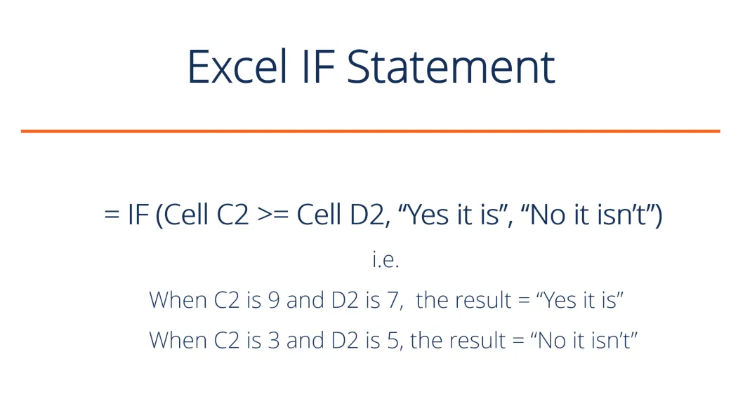
Website:  https://support.microsoft.com/en-us/office/if-function-69aed7c9-4e8a-4755-a9bc-aa8bbff73be2 As a Project Analyst, I used IF statements to check how much credits were generated for a single employee in 2020. The if statements are used to check several things and can produce a result if the condition turns out true or false. When I joined the team, there was already a template that utilized embedded IF statements paired with other functions like vlookup because there were several tabs within one excel file.  Below, I decided to play around with several IF statements and concluded with a SUMIF to calculate the credit generated for a single employee in 2020.  The main idea with my formulas is to find at what quarter does the employee's gross pay goes over 10k. In this case for employee John, it was Q3. Therefore, I calculated 50% of his Q1 and Q2 gross pay to be credit generated. In Q3, he went over. Since I know 5,000 is the maximum generated credit for 2020, then ...

Proper Website:  https://support.microsoft.com/en-us/office/proper-function-61db8dc3-a6ca-456e-ab1b-e93ad47da569#:~:text=Capitalizes%20the%20first%20letter%20and,text%20string%20to%20lowercase%20letters. PROPER(text) Text is text enclosed in quotation marks, a formula that returns text, or a column reference containing the text you want to partially capitalize. Trim Website:  https://support.microsoft.com/en-us/office/trim-function-410388fa-c5df-49c6-b16c-9e5630b479f9 TRIM(text) The TRIM function syntax has the following arguments: Text Required. The text from which you want spaces removed. As a Project Analyst, I used both the proper and trim functions to clean up payroll excel files of employee names. Not only is this important for making your work look clean, but also trim is essential for making sure your conditional formatting worked. If "John " (with a space) and "John" (no space) are checked for exact match using conditional formatting, it will not hig...

 Website:  https://support.microsoft.com/en-us/office/subtotal-function-7b027003-f060-4ade-9040-e478765b9939 SUBTOTAL(function_num,ref1,[ref2],...) The SUBTOTAL function syntax has the following arguments: The number 1-11 or 101-111 that specifies the function to use for the subtotal. 1-11 includes manually-hidden rows, while 101-111 excludes them; filtered-out cells are always excluded. When I work on unbilled media accruals as a Finance & Accounting Specialist, I used the subtotal function and 109 to sum up the filtered report for reporting the upcoming month's expected billing.  I turned my data set into a table with Ctrl + T and then inserted a slicer for easy filtering. Feel free to open the workbook and use the slicer to see how it works with the subtotal formula.  You can find the subtotal of unbilled gross for a single media type or multiple media types by selecting the ones you desire. The multi-select tool allows for the user to select multiple options....

Website:  https://support.microsoft.com/en-us/office/sumif-function-169b8c99-c05c-4483-a712-1697a653039b SUMIF(range, criteria, [sum_range]) Website:  https://support.microsoft.com/en-us/office/countif-function-e0de10c6-f885-4e71-abb4-1f464816df34 =COUNTIF(Where do you want to look?, What do you want to look for?) As a Finance & Accounting Specialist, I used the sumif to sum up the amount Innocean spent for a specific vendor to help with advertising for our client. I used the countif to sum up the number of transactions there are for a specific vendor on a bank statement for a certain month. This is the very first step that is required for credit card bank reconciliation process to ensure all transactions and costs are accounted for. The treasury provides us with the bank statement in an excel format.  On the bank statement, it will not just say "LINKEDIN" but will contain more verbage within a cell. For example, it may say "LINKEDIN.REFID.12345." Before I use t...

As a Finance & Accounting Specialist, I need to check that the finalized client invoices match our billing summary gross amount. I created this conditional formatted list to keep track what match and did not match. Then, I would make the appropriate changes to the commission rates so they would match. Our system Mediaocean does not always calculate at the exact commission rate due to rounding so that is why we must go through this process to ensure our numbers on Excel match with what we are sending to the client. Data --> Data Validation Make it a list and enter your 2 options Conditional Formatting --> Manage Rules Set the cell to be highlighted green when cell says "Match" and highlighted red when cell says "Do Not Match" See below what it will look like:

To view any excel workbook and the formulas within their cells, please click on the bottom right icon. Also, once I learned about the FORMULATEXT function so I starting utilizing that at some point so you can see the whole formula without having to click into a cell.  Note the following: 1) All numbers are made up; I often use the RANBETWEEN() function to randomize numbers. It allows you to restrict the randomized number with a min and max value. 2) On the Excel Blogspot article, you can utilize the dropdowns and filters. However, once you open he excel workbook with the bottom right icon, it no longer allows you that option. For example, look at the article below and try the dropdown and filters on the blogspot website vs. opening it in an excel workbook using bottom right icon. Article:  GETPIVOTDATA

Website: https://support.microsoft.com/en-us/office/xlookup-function-b7fd680e-6d10-43e6-84f9-88eae8bf5929 The XLOOKUP function searches a range or an array, and then returns the item corresponding to the first match it finds. If no match exists, then XLOOKUP can return the closest (approximate) match. =XLOOKUP(lookup_value, lookup_array, return_array, [if_not_found], [match_mode], [search_mode]) As a Finance & Accounting Specialist, I used the xlookup for each month's UC Davis Health billing. There are different ATB ("Authorization to Buy") numbers, estimate numbers, media types, and ATB names. Our goal is to to see how much we are billing for each ATB number to make sure we are in budget and to check if we are billing enough for each ATB, which we can be summarized using a pivot table of the full report data. Also, if "N/A" returns, then I know there is either a new ATB that I would request more info from the media team. However, as mentioned in its definit...

Website: https://support.microsoft.com/en-us/office/vlookup-function-0bbc8083-26fe-4963-8ab8-93a18ad188a1 A Vlookup Function says: =VLOOKUP(What you want to look up, where you want to look for it, the column number in the range containing the value to return, return an Approximate or Exact match – indicated as 1/TRUE, or 0/FALSE) My most common usage of vlookup was using it to ensure I did not pay invoices from last week. As a Finance & Accounting Specialist at Innocean, I created the Wienerschnitzel payment request every Wednesday. We use our system Mediaocean to pull the AP import file report in csv format that will show all invoices that were reconciled. However, since the report is pulled from Wednesday of last week to Wednesday today, then it is possible it will generate the same invoices from last week's payment request.  In the example below, I used the vlookup and FALSE exact match to find out that invoice 897 and 105 was already paid in last week's payment request....